AD8307 Data Sheet
Rev. E | Page 10 of 24
The most widely used reference in RF systems is decibels above
1 mW in 50 , written dBm. Note that the quantity (P
IN
– P
0
) is
just dB. The logarithmic function disappears from the formula
because the conversion has already been implicitly performed
in stating the input in decibels. This is strictly a concession to
popular convention; log amps manifestly do not respond to power
(tacitly, power absorbed at the input), but rather to input voltage.
The use of dBV (decibels with respect to 1 V rms) is more precise,
though still incomplete, because waveform is involved as well.
Because most users think about and specify RF signals in terms
of power, more specifically, in dBm re: 50 , this convention is
used in specifying the performance of the AD8307.
PROGRESSIVE COMPRESSION
Most high speed, high dynamic range log amps use a cascade of
nonlinear amplifier cells (see Figure 22) to generate the logarithmic
function from a series of contiguous segments, a type of piecewise
linear technique. This basic topology immediately opens up the
possibility of enormous gain bandwidth products. For example,
the AD8307 employs six cells in its main signal path, each having
a small signal gain of 14.3 dB (×5.2) and a −3 dB bandwidth of
about 900 MHz. The overall gain is about 20,000 (86 dB) and
the overall bandwidth of the chain is some 500 MHz, resulting
in the incredible gain bandwidth product (GBW) of 10,000 GHz,
about a million times that of a typical op amp. This very high
GBW is an essential prerequisite for accurate operation under
small signal conditions and at high frequencies. In Equation 2,
however, the incremental gain decreases rapidly as V
IN
increases.
The AD8307 continues to exhibit an essentially logarithmic
response down to inputs as small as 50 V at 500 MHz.
V
X
V
W
STAGE 1 STAGE 2 STAGE N–1 STAGE N
A A A A
1082-022
Figure 22. Cascade of Nonlinear Gain Cells
To develop the theory, first consider a scheme slightly different
from that employed in the AD8307, but simpler to explain and
mathematically more straightforward to analyze. This approach
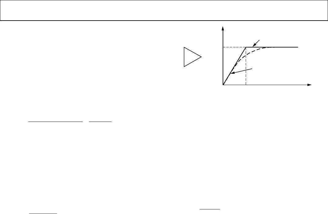
is based on a nonlinear amplifier unit, called an A/1 cell, with
the transfer characteristic shown in Figure 23.
The local small signal gain δV
OUT
/δV
IN
is A, maintained for all
inputs up to the knee voltage E
K
, above which the incremental
gain drops to unity. The function is symmetrical: the same drop
in gain occurs for instantaneous values of V
IN
less than –E
K
. The
large signal gain has a value of A for inputs in the range −E
K
≤
V
IN
≤ +E
K
, but falls asymptotically toward unity for very large
inputs. In logarithmic amplifiers based on this amplifier function,
both the slope voltage and the intercept voltage must be traceable
to the one reference voltage, E
K
. Therefore, in this fundamental
analysis, the calibration accuracy of the log amp is dependent
solely on this voltage. In practice, it is possible to separate the
basic references used to determine V
Y
and V
X
and, in the case of
the AD8307, V
Y
is traceable to an on-chip band gap reference,
whereas V
X
is derived from the thermal voltage kT/q and is later
temperature corrected.
1082-023
SLOPE = A
SLOPE = 1
OUTPUT
AE
K
E
K
0
INPUT
A/1
Figure 23. A/1 Amplifier Function
Let the input of an N-cell cascade be V
IN
, and the final output
be V
OUT
. For small signals, the overall gain is simply A
N
. A
six-stage system in which A = 5 (14 dB) has an overall gain
of 15,625 (84 dB). The importance of a very high small signal
gain in implementing the logarithmic function has been noted;
however, this parameter is only of incidental interest in the design
of log amps.
From this point forward, rather than considering gain, analyze
the overall nonlinear behavior of the cascade in response to a
simple dc input, corresponding to the V
IN
of Equation 1. For
very small inputs, the output from the first cell is V
1
= AV
IN
.
The output from the second cell is V
2
= A
2
V
IN
, and so on, up to
V
N
= A
N
V
IN
. At a certain value of V
IN
, the input to the Nth cell,
V
N − 1
, is exactly equal to the knee voltage E
K
. Thus, V
OUT
= AE
K
and because there are N − 1 cells of Gain A ahead of this node,
calculate V
IN
= E
K
/A
N − 1
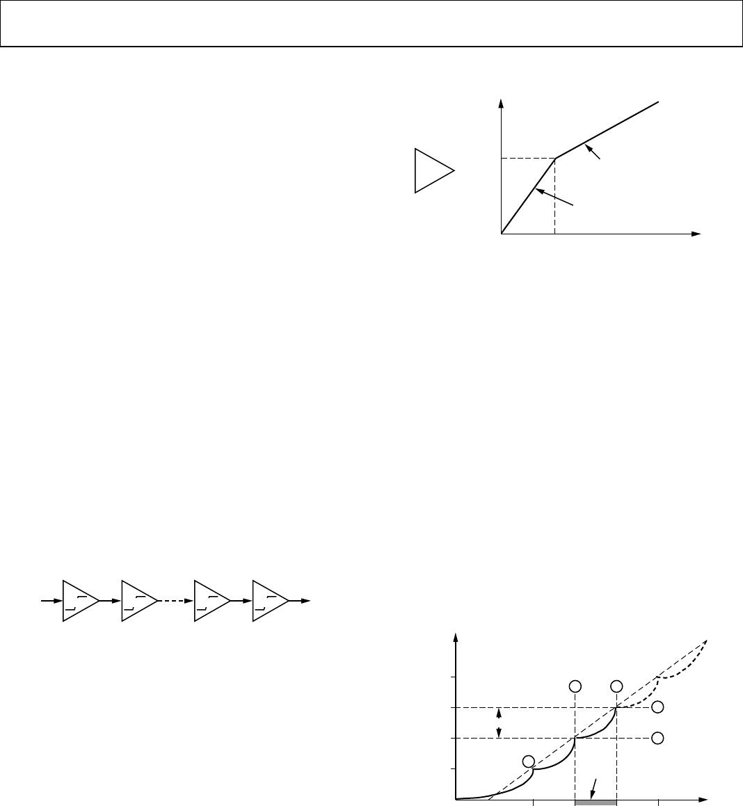
. This unique situation corresponds to
the lin-log transition (labeled 1 in Figure 24). Below this input,
the cascade of gain cells acts as a simple linear amplifier, whereas
for higher values of V
IN
, it enters into a series of segments that
lie on a logarithmic approximation (dotted line).
RATIO
OF A
2
1
3
3
2
E
K
/A
N–1
E
K
/A
N–2
E
K
/A
N–3
E
K
/A
N–4
LOG V
IN
(4A–3) E
K
V
OUT
(3A–2) E
K
(2A–1) E
K
AE
K
0
(A–1) E
K
01082-024
Figure 24. First Three Transitions
Continuing this analysis, the next transition occurs when the
input to the N − 1 stage just reaches E
K
, that is, when V
IN
=
E
K
/A
N − 2
.
The output of this stage is then exactly AE
K
, and it is
easily demonstrated (from the function shown in Figure 23) that
the output of the final stage is (2A − 1)E
K
(labeled 2 in Figure 24).
Thus, the output has changed by an amount (A − 1)E
K
for a
change in V
IN
from E
K
/A
N − 1
to E
K
/A
N − 2
, that is, a ratio change of A.
At the next critical point (labeled 3 in Figure 24), the input is